
Implementing a Session-based kNN in Python
August 2, 2020
As the troves of easily accessible information continue to grow exponentially, enabling users to comfortably explore such complex information landscapes becomes increasingly important. This, in essence, is the job of recommender systems. In this post, I will implementing one such system in the context of session-based music consumption. In the era of on-demand music streaming, we face some unique challenges; ranging from the inherent abundance of music and its disposable nature to its unique consumption. Notably, however, experiences from session-based music recommendation can be extrapolated to other fields similarly deailng with series or sequences of data, e.g. e-commerence and finance.
Introduction
A conventional recommender system typically ignores sequential information as it seeks to infer static relevancy between users and items. Systems based on matrix factorisation, for instance, may be effective at modelling the general preferences of a user by analysing their past interactions with the system, but they do not model the order of these interactions. Such static representation is problematic because it fails to accommodate both short- and long-term preferences, and, as a direct consequence, does not adequately account for how a given user’s preferences naturally evolve over time. While the speed at which preferences evolve depends on the specific context—it is reasonable to assume, for instance, that it takes longer for your preferences to evolve when watching movies than when enjoying music simply due to the time it takes to consume a single item—being able to account for changes is key to producing good recommendations. Accordingly, in the context of session-based recommenders, conventional techniques are often subpar.
An early step towards better accommodating sessions using session-based collaborative filtering (SBCF) was proposed by Park et al. in Session-Based Collaborative Filtering for Predicting the Next Song [1]. Instead of creating user profiles as many conventional systems do, Park et al. create session profiles. This, effectively, ensures that only information inherently relevant to the current session can affect the next-item recommendation. Whilst this obviously does not accommodate nor account for the long-term preferences of a user, SSCF should, in theory, enjoy increased accuracy in predicting short-term, session-based preferences by referring to similar sessions.
In other words; SSCF seeks to exploit the fact that a session consisting of, say, ambient music is more likely to share next-item songs with other ambient sessions than diverge into to, say, songs most commonly seen in punk sessions. In this post, we will implement a multi-processing version of the SSCF model as proposed by Park et al. using Python.
Note that the subtle yet distinct difference between session-based and session-aware recommendation. The former denotes the problem in which only the current sequence of actions by a giver user within some specified interval is known. The latter seeks to predict what happens next by modelling a user’s short-term preferences using past sessions alongside implicit feedback given to the system by the user during the current session; effectively exploiting any dynamic, sequential patterns present in the user’s behaviour. In this post, we are dealing with session-based recommendation.
Problem Definition
We define a user’s complete listening history $H$ as a sequence of tuples $(user, track, timestamp)$. A session is composed of a set of tuples from $H$ within a given interval (e.g. one hour). Assuming that we have $n$ tracks and $m$ sessions, the set of tracks can be defined as $T = {t_1, t_2, …, t_n}$ and the set of sessions $S = {s_1, s_2, …, s_m}$. We consider the profile of a session $s$ as the pairs of tracks and their associated playcounts. Accordingly, in the recommendation matrix, rows represent session profiles and columns represent tracks. The individual cells contain the frequency a given track was played in a given session.
In order to predict the ratings of the next track $i$ in the current session $s$, we compute:
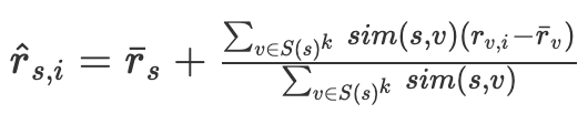
$S(s)^k$ represents the $k$-th session neighbours for the current session $s$. $\overline{r_{s}}$ and $\overline{r_{v}}$ represent the average rating for sessions $s$ and $v$ under comparison, respectively. $r_{v,i}$ represents the frequency a track $i$ is played in session $v$, and, finally, $sim(s,v)$ represent the similarity between sessions $s$ and $v$. In this specific implementation, we will be applying cosine similarity, though other similarity measures could also be used. Note that the original paper presents the above in a slightly different manner, but the end-result is the same. I find the above formulation easier to grasp.
Dataset
I will be working with a customised version of the Lastfm-1K dataset originally collected by Òscar Celma (available at http://ocelma.net/MusicRecommendationDataset/lastfm-1K.html). The original dataset contains the complete listening history of 992 unique Last.fm users tracked between 2005 and 2009. The version employed in this post has been augmented with community-created for each individual track. Due to shortcomings with the Last.fm API, tags have been obtained by scraping each dedicated track page directly. Additional informationm, including download links for the complete set, is available here.
Implementation
We start by constructing our SKNN matrix:
def construct_sknn_matrix(train_sessions, num_of_tracks):
    sessions = train_sessions.tracks.values.tolist()
    sknn_mat = sparse.lil_matrix((len(sessions), num_of_tracks),
                                 dtype=np.int16)

    for i, session in enumerate(sessions):
        unique_tracks = list(set(session))
        track_plays = dict(
            zip(unique_tracks, [0] * len(unique_tracks)))
        for track in session:
            track_plays[track] += 1
        for key in track_plays:
            sknn_mat[i, key - 1] = track_plays[key]

    return sknn_mat.tocsr()
In constructing our sknn_mat (SKNN-matrix), we convert our training sessions to a list. We then instantiate sknn_mat using scipy’s sparse.lil_matrix [2]. This row-based list-of-lists sparse matrix allows us to construct a sparse matrix incrementally. Note that we deliberately set the dtype as np.int16 to minimise the size of sknn_mat. Realistically, np.int8 is likely sufficient, but on the odd chance that a song has been played more than 256 times in a single session, we use np.int16. The shape of sknn_mat is (len(sessions), len(tracks)).
We then iterate through all our sessions and extract the list of unique tracks and their playcounts. Then, for each unique track in the session, we update our sknn_mat for the given session (i.e. row) and update the playcounts of all tracks. Note that the vast majority of cells will hold the value $0$ as only a small subset of the available songs will ever be played during a single session—hence why we opt for a sparse matrix format. We finish by converting sknn_mat to a CSR matrix such that we can work with it more efficiently moving forward. This format can, moreover, easily be dumped to disk as .npz. This is particularly helpful in that we need only create the matrix once and subsequently generate all the recommendations we need using this matrix. Of course, if our training data changes, we need to update our matrix accordingly.
Evaluation
A more complicated task is actually evaluating the performance of our SKNN. In essence, given an arbitrary target session and the task of predicting its next track, we need to iterate through every session (i.e. row) in sknn_mat, compute the similarity between that and our target session, note which rows have the highest similarity, and finally return top $k$ rows. In this example, we set $k = 10$.
def eval_sknn(sknn_matrix, start_idx, end_idx, num_of_tracks,
              nn=10, topk=10, batch_size=1000):

    batches = []
    # Generate list of batches for each core.
    for i in range(start_idx, end_idx, batch_size):
        batches.append(test_sessions_list[i:i + batch_size])

    total = 0
    correct = 0
    for batch in batches:
        target_dict = {}
        test_matrix = sparse.lil_matrix((len(batch), num_of_tracks),
                                        dtype=np.int16)

        # Iterate all tracks in a batch and fill target_dict.
        for i, session in enumerate(batch):
            input_tracks = session[:-1]
            target = session[-1] - 1
            target_dict[i] = target
            unique_tracks = list(set(input_tracks))
            track_plays = dict(
                zip(unique_tracks, [0] * len(unique_tracks)))

            for track in input_tracks:
                track_plays[track] += 1
            for key in track_plays:
                test_matrix[i, key - 1] = track_plays[key]

        # Prepare matrices for evaluation.
        test_matrix = test_matrix.tocsr()
        similarity_matrix = cosine_similarity(
          test_matrix, sknn_matrix, dense_output=False)
        test_mean_ratings = test_matrix.mean(axis=1)

        ...
A couple of things happen in the above snippet. Note that we opt for the creation of batches as our intended dataset is relatively large and we wish to utilise all available cores at our disposal. This is likely worthwhile even if your dataset is smaller. The start_idx and end_idx thus define the interval of our training sessions assigned to a single core. We further split that interval into batches. If you are dealing with a small dataset, there is likely no need to create individual batches like this. We then iterate through our list of batches. The first thing we do is to construct our target_dict which holds the correct next-track for the given session.
We proceed to construct our test_matrix using all tracks in the given batch as columns, each session in the batch as rows, and each cell as the playcount of track $x$ in session $y$ similar to our sknn_matrix. Once done, we compute the similarity_matrix which, in this instance, happens to be the cosine similarity between our test_matrix and sknn_matrix. We conclude the preparatory steps by computing the mean track ratings (i.e. playcounts), and proceed to the actual evaluation.
        ...
        for i in range(len(batch)):
            # Grab neighbours.
            neighbours = np.argpartition(
              similarity_matrix[i].toarray()[0], -nn)[-nn:]
            # Compute the rating denominator.
            rating_denom = similarity_matrix[i, neighbours].sum()
            # Compute mean test/train ratings.
            test_mean_rating = test_mean_ratings[i].item()
            train_mean_ratings = sknn_matrix[neighbours].mean(axis=1)
            # Compute similarities.
            train_simililarities = similarity_matrix[i, neighbours]
            # Grab ratings for neighbours.
            neighbour_ratings = sknn_matrix[neighbours]
            # Compute scores for each track.
            track_scores = np.multiply(
                neighbour_ratings - train_mean_ratings,
                train_simililarities.toarray().squeeze(0)\
                [:, np.newaxis]).sum(axis=0)
            # Compute the track ratings.
            track_ratings = track_scores / rating_denom\
                            if rating_denom != 0 else track_scores

            track_scores = test_mean_rating + track_ratings
            # Slice to grab top-k tracks.
            topk_tracks = np.argpartition(
                np.asarray(track_scores)\
                .reshape(-1), -topk)[-topk:]

            total += 1
            if target_dict[i] in topk_tracks:
                correct += 1

	results_queue.put((correct, total))
In evaluating our SKNN model, we iterate through every session in each batch. We find its top-$k$ neighbours—that is, the session the most similar to the one we are currently looking at. In practice, this is determined by looking at the output from our cosine similarity computations and finding those with the highest values.
Putting It Together
With the construction of our matrix and subsequent evaluation in place, all we have left is to read our data, create our testing and training splits, and otherwise separate the workload to each of our cores. Note that in this specific implementation, I am using a machine with 32 cores available. Please remember to adjust the parameter to a number suitable for your system.
trained_sknn = None
test_sessions_list = None
results_queue = mp.Queue()

def generate_batch(sessions, batch_size):
    for i in range(0, len(sessions), batch_size):
        yield sessions[i:i + batch_size]

if __name__ == "__main__":
    NUM_OF_CORES = 32
    TRAIN_TEST_SPLIT = 0.7

    # Load all data as dataframes.
    ABSOLUTE_PATH = str(Path(__file__).resolve().parents[1].absolute())\
                    + "{0}data{0}".format(os.sep)
    with open(ABSOLUTE_PATH + "sessions.json", "r") as source:
        sessions = pd.read_json(source, orient="index")

    with open(ABSOLUTE_PATH + "tracks.json", "r") as source:
        tracks = pd.read_json(source, orient="index")
        NUM_OF_TRACKS = len(tracks)

    with open(ABSOLUTE_PATH + "users.json", "r") as source:
        users = pd.read_json(source, orient="index")

    # Create the training and testing split.
    train_sessions, test_sessions = get_split(
        users, sessions, TRAIN_TEST_SPLIT)
    #  If your data does not contain a 'tags' column, remove this.
    test_sessions.drop("tags", axis=1, inplace=True)
    test_sessions_list = test_sessions.tracks.values.tolist()

    # Allow both training and evaluations.
    if sys.argv[1] == "train":
        trained_sknn = train_sknn(train_sessions, NUM_OF_TRACKS)
        sparse.save_npz("trained_sknn_tf.npz", trained_sknn)
    if sys.argv[1] == "eval":
        # Load the saved training sparse matrix; in csr format.
        trained_sknn = sparse.load_npz("trained_sknn_tf.npz")

    TOTAL = len(test_sessions_list)
    SESSIONS_PER_CORE = math.ceil(TOTAL / NUM_OF_CORES)

    # We test a broad range of neighbours and top-k values.
    # Typically, performance will stagnate at some neighbour
    # value. In this case, around 100-125. This depends
    # entirely on your data, so edit accordingly.
    neighbours = [10, 25, 50, 75, 100, 125, 150]
    topk = [10, 20, 30, 40, 50]
    for neighbour in neighbours:
        for k in topk:
            processes = []
            for i in range(NUM_OF_CORES):
                process_start = i * SESSIONS_PER_CORE
                process_end = process_start + SESSIONS_PER_CORE
                p = mp.Process(target=eval_sknn,
                                args=(trained_sknn, process_start,
                                      process_end, NUM_OF_TRACKS,
                                      neighbour, k))
                processes.append(p)
                p.start()
                print("Started process", i)

            # Wait for all processes to finish.
            for p in processes:
                p.join()

            # Combine results; compute performance.
            results = [results_queue.get() for p in processes]
            correct = sum([pair[0] for pair in results])
            total = sum([pair[1] for pair in results])
            cumulative_rank = sum([pair[2] for pair in results])

            hit_ratio = correct / total
            print("Hit ratio @ {}: {} ({} hits in {} samples)"\
                 .format(k, hit_ratio, correct, total))

            mrr = cumulative_rank / total
            print("Mean Reciprocal Rank @ {}: {}"\
                 .format(k, mrr))

            # Write results to disk.
            with open("sknn_results.txt", "a") as out:
                out.write("Hit ratio @ {}: {} ({} hits in {} samples): {} neighbours\n"\
                        .format(k, hit_ratio, correct, total, neighbour))
                out.write("Mean Reciprocal Rank @ {}: {}\n".format(k, mrr))
The get_split function looks as follows:
def get_split(user_data, session_data, train_split):
    def split_user_sids(sids):
        split_index = math.ceil(len(sids) * train_split)
        return sids[:split_index], sids[split_index:]

    def get_subsessions(pairs):
        subsessions = {}
        counter = 0
        for session in pairs:
            session_tracks = session[0]
            session_tags = session[1]
            for i in range(1, len(session_tracks)):
                subsessions[counter] = {"tracks" : session_tracks[:i+1],
                                        "tags" : session_tags[:i+1]}
                counter += 1

        return pd.DataFrame.from_dict(subsessions, orient="index")


    split = user_data["sessions_subset"].apply(split_user_sids)
    train_sids = [item for sublist in split.tolist() for item in sublist[0]]
    test_sids = [item for sublist in split.tolist() for item in sublist[1]]

    train_session_data = session_data.loc[train_sids]
    test_session_data = session_data.loc[test_sids]

    # Prepare training data.
    train_tracks = train_session_data.track_idxs.values.tolist()
    train_tags = train_session_data.tags_idxs.values.tolist()
    train_pairs = list(zip(train_tracks, train_tags))

    # Prepare testing data.
    test_tracks = test_session_data.track_idxs.values.tolist()
    test_tags = test_session_data.tags_idxs.values.tolist()
    test_pairs = list(zip(test_tracks, test_tags))

    return get_subsessions(train_pairs), get_subsessions(test_pairs)
Note that for sake of simplicity, a validation set is not generated. The complete code includes this functionality, and the above function thus looks slightly different. Depending on your use-case, apply whichever is appropriate.