A recurrent neural network, or RNN, is a relatively simple yet powerful extension to conventional feed-forward neural networks. Indeed, unlike conventional networks, RNNs can accommodate variable-length input sequences (as well as produce variable-length output sequences). This is especially powerful when dealing with series or sequences as chances are neighbouring entries influence the current entry. RNNs can capture such relationships. Accordingly, in recent years, RNNs have produced increasingly promising results in numerous machine learning tasks; especially those featuring varying input and output lengths such as machine translation. The central component allowing the networks to achieve these results is the recurrent unit, or hidden state, whose activation at each time step $t$ is dependent on that of the previous time step $t-1$. That is, given a variable-length input sequence $x=(x_1,x_2,…,x_n)$, an RNN updates its recurrent hidden state $h_t$ by

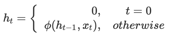
where $\phi$ is a some non-linear function. Traditionally, the recurrent hidden state is updated by computing $h_t = f(Wx_t + Uh_{t-1})$ where $f$ is a smooth, bounded function; $W$ is the set of weights for the input $x_t$; and $U$ is the set of weights from the previous hidden state $h_{t-1}$. The RNN may also have an output $y=(y_1,y_2,…,y_m)$, which, again, can be of variable-length. If you are entirely new to the concept of RNNs, consider checking this post before proceeding.

However, RNNs are not perfect. Ultimately, their ability to capture long-range dependencies diminishes the longer the input becomes. Bengio et al. [2012, 1994] showed this to be a result of the gradients (error signals) eventually vanishing or, more rarely, exploding. The former is caused by the fact that backpropagation computes gradients using the chain rule—something which means that $k$ gradients are multiplied in $k$ layers, ultimately decreasing the signal exponentially to the point where the front layers either train very slowly, or stop training all together. The latter, exploding gradients problem refers to the opposite, and much rarer, instance in which long-range components grow exponentially more than short-range ones due to a large increase in the norm of the gradient during training.

As such, gradient-based optimisation methods struggle—both because of the variations in gradient magnitudes, and because the effect(s) of long-range dependencies can be hidden by the effect(s) of short-range dependencies. Now, if we are strictly interested in short-range dependencies, this might not matter much. However, in most real-world data, long-range dependencies tend to be present. Adequately capturing such dependencies, in addition to accommodating short-range dynamics, will thus almost always improve accuracy. We, therefore, need to upgrade our RNNs. We fundamentally have two ways in which we can do that: We can either (1) devise a better learning algorithm; or (2) design a more sophisticated activation function. In this post, we will examine the latter approach in the form of the Gated Recurrent Unit (GRU) as proposed by Cho et al. [2014].

Note that an earlier solution to the vanishing gradients problem is the so-called Long Short-term Memory (LSTM) units proposed by Hochreiter and Schmidhuber [1997]. If you are interested in learning more about LSTMs, please refer to this post. Generally, both GRUs and LSTMs outperform vanilla RNNs if long-range dependencies are important, but might also outperform even when sequences are relatively short. However, whether we should choose GRU or LSTM ultimately depends on our data and model. Advantages and disadvantages of both approaches are discussed at the end of this post. Worth also noting is that we are strictly concerning ourselves with the issue of the vanishing gradients problem: Neither LSTMs nor GRUs solve the issue of exploding gradients as discussed by Bengio et al. [2012].

Introducing the Gated Recurrent Unit

As previously noted, GRUs are designed to address the vanishing gradients problem present in conventional recurrent neural networks. In other words: GRUs are designed to both remember and—perhaps more importantly—forget better. The underlying idea is that by creating a more sophisticated activation function consisting of an affine transformation followed by element-wise non-linearity using gating units, long-range dependencies can be captured. That was quite the mouthful, and it is simpler than it might sound! No worries. Your brain taking note of this important—and hopefully consoling—piece of information, by the way, is a little like how GRUs operate.

What the above description really says is that we enable each recurrent unit to adaptively capture dependencies across different time steps. In practice, GRUs achieve this by incorporating special gating mechanisms which modulate the flow of information inside each unit. Specifically, a GRU consists of an update gate and a reset gate. If you are familiar with LSTM units, you will note that GRUs do not feature a separate memory cell. If you are not familiar with LSTMs, no need to worry; both solutions are discussed at the end of this post. In essence though, both the update and reset gate are really just vectors whose job we make it to determine which information should be passed as output. What makes them special is that we can train them using sigmoid activation functions to retain certain information relevant to our model for longer periods of time—or, conversely, completely forget some information deemed irrelevant for our model.

The below illustration shows a single GRU. You might have seen similar illustrations with multiple units chained together. While this is helpful in visualising how GRUs are just another variation of RNNs, it can also complicate the matter. What is worth remembering is how a single cell, like the one below, takes as input information (i.e. a hidden state) from its predecessor, and passes a modified version of the same information to its successor. This is exactly the same process as in conventional RNNs. The difference, of course, lies in how we modify the hidden state. In this post, we focus on a single GRU and incrementally step through the flow of information.

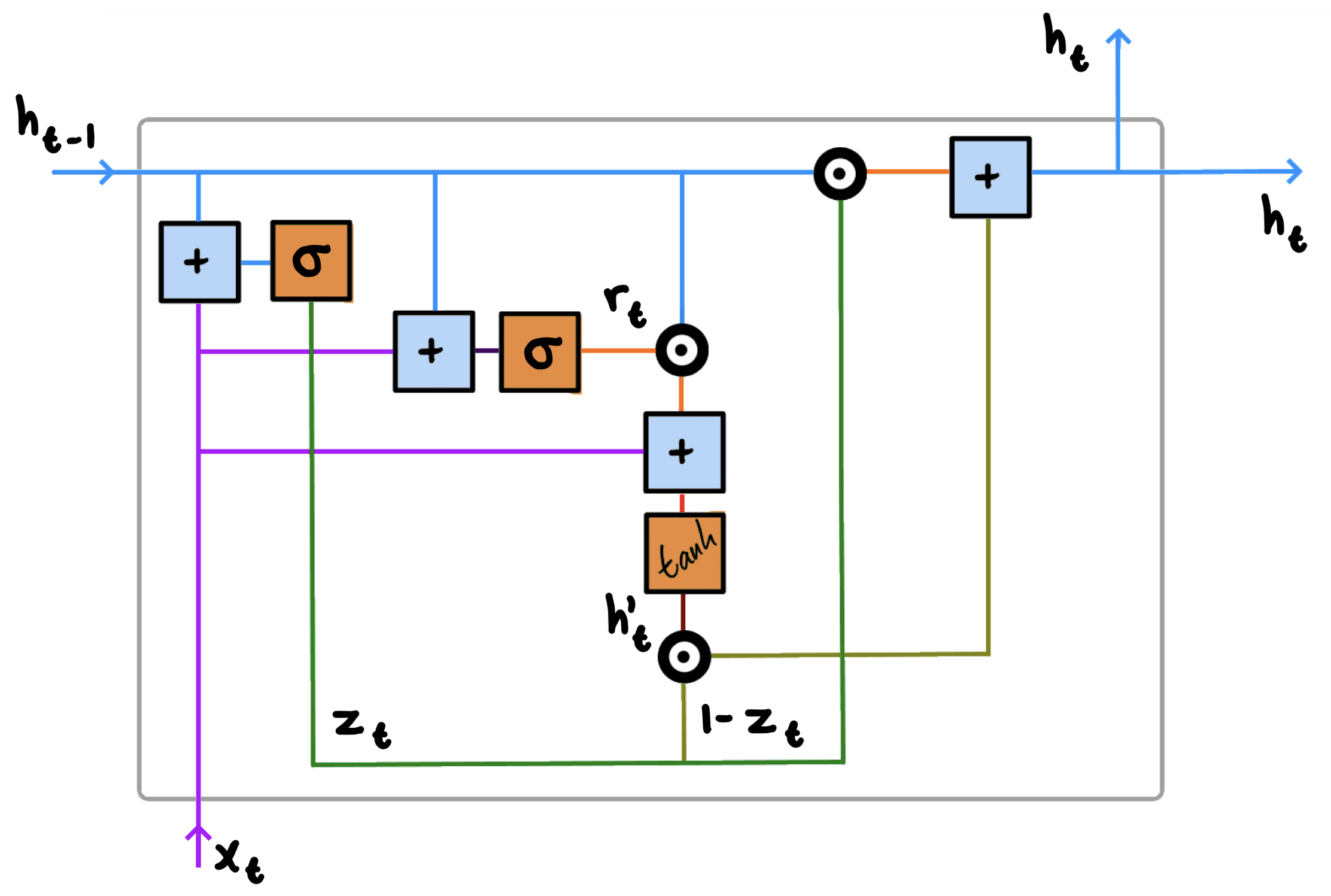
This might look somewhat confusing at first glance, but bear with me for a minute. If we start by introducing the notations before incrementally going through the flow, we note the following:

The plus operation is literally adding two elements together. The $\sigma$ and $\tanh$ functions are both activation functions for their respective gates. While these are covered in greater detail shortly, please refer to this tutorial if you would like more information. The Hadamard-product operation denotes element-wise multiplication of matrices. Additionally, you will find the variables $h$, $x$, $z$, $r$, and $t$. These, too, will be covered in greater detail below. What is worth emphasising, however, is how the coloured lines represent the flow of information throughout the unit.

1. Update Gate $z$

All GRUs take two inputs: $h_{t-1}$ and $x_t$.

$h_{t-1}$ is the hidden state, or activation, $h$ from the previous time step $t-1$. In most cases, this value is passed along from another GRU, but it may also come from another component of our network. Regardless of where it comes from though, $h_{t-1}$ is an encoding of all information prior to the current state. $x_t$, on the other hand, represents the input from the current time step $t$. Similar to RNNs, when dealing with the very first step, we naturally do not have a prior hidden state vector available, and typically initialise using all $0$’s instead.

In some instances, we might very well be interested in accounting for all past information, but in most cases, everything is not necessarily going to be equally relevant at all times. What you ate last week, for instance, is perhaps not as indicative of what you will be eating tonight as what you ate yesterday. On the other hand, if we are recommending movies, it does not make sense to recommend the movie we just watched either. As such, we need a mechanism to determine how much past information we should pass along. This is the job of the update gate.

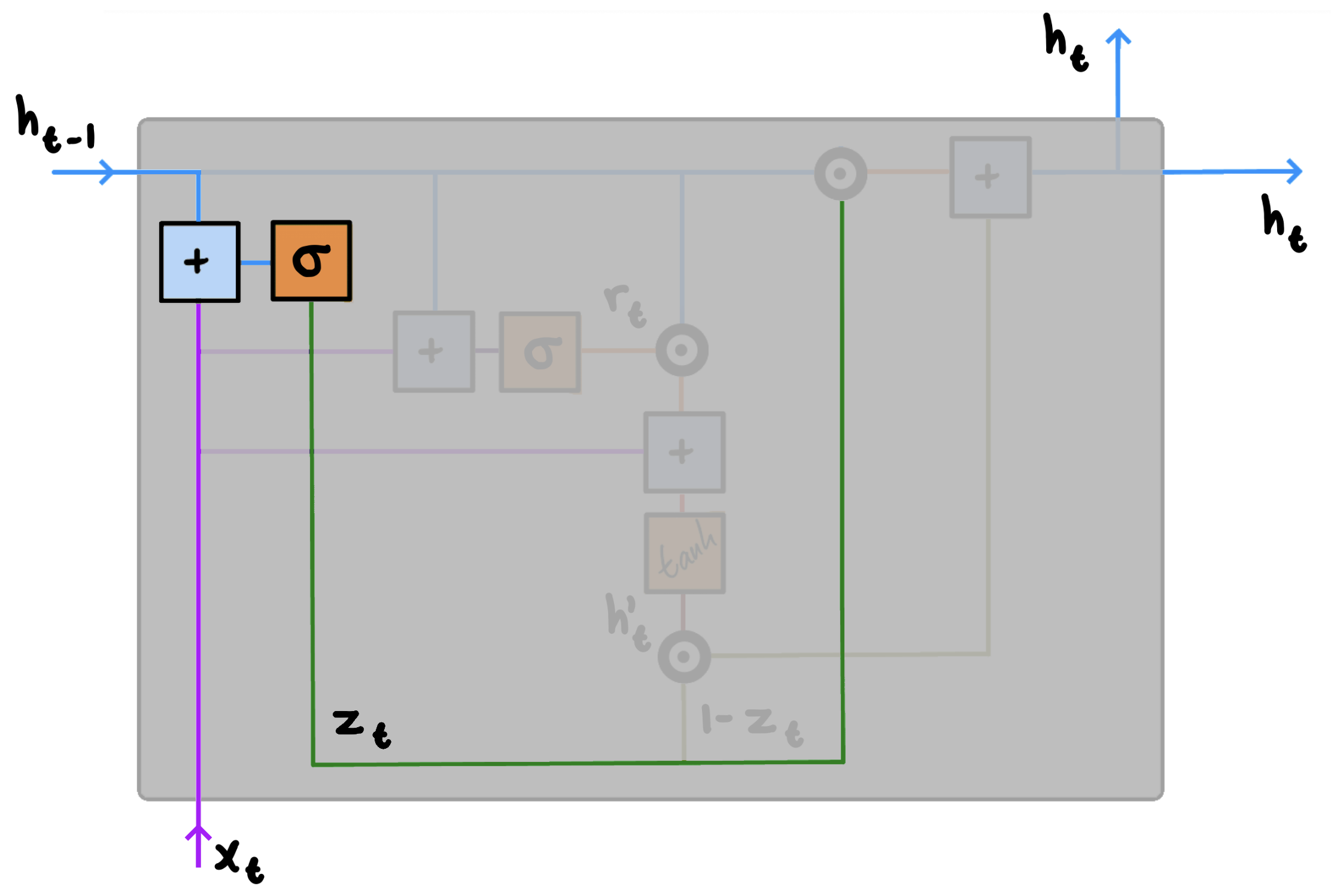
We compute the update gate $z$ for time step $t$ using:

When $x_t$ is plugged into the network unit, it is multiplied by its own weight $W_z$. This also applies to the input $h_{t-1}$ we obtain from the previous step, which is similarly multiplied by its own weight $U_z$. The results are then added together after which a sigmoid activation function is applied to squash the result between 0 and 1. Occasionally, some information will diminish in importance following the squash, though all past information could also be passed along largely unchanged in importance. This all depends on our data and is exactly the behaviour we want. The notion of taking a linear sum between the existing state and the new state is similar to that of LSTM units. However, unlike LSTMs, GRUs have no mechanism to control the degree to which its state is exposed. Instead, GRUs expose the whole state every step. In other words: At each time step $t$, we consider all available information.

2. Reset Gate $r$

The reset gate is the mechanism by which GRUs forget. That is, the job of the reset gate is to determine how much past information a given unit should retain. This might sound similar to the update gate, but there is a distinct difference: The update gate determines what of both old and current information to pass along—the reset gate determines how much old information to forget using the new information $x_t$.

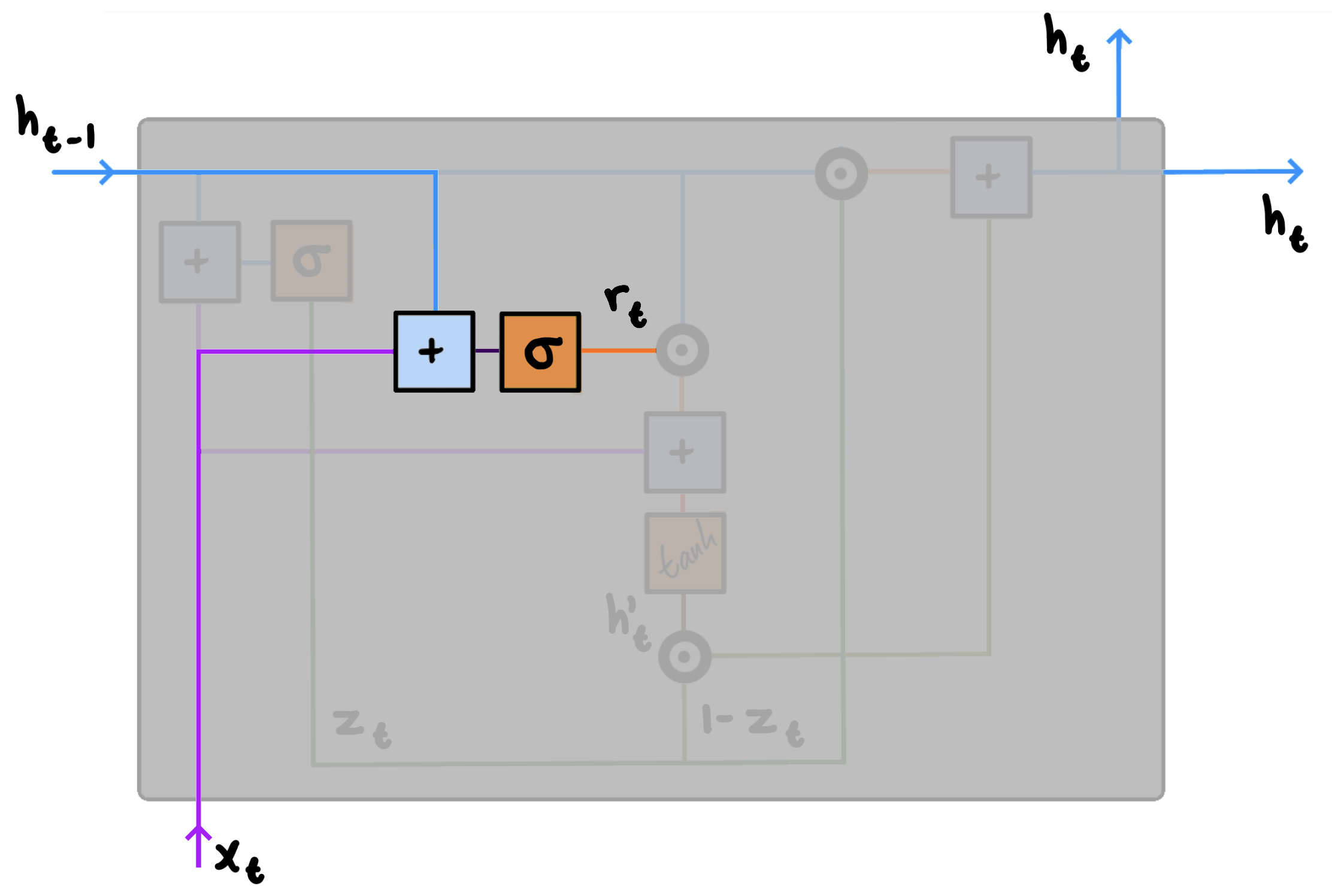
We compute the reset gate $r$ for time step $t$ using:

Similar to the update gate, when $x_t$ is plugged into the network unit, it is multiplied by its own weight $W_r$, and $h_{t-1}$ is multiplied by its own weight $U_r$. Once done, the results are added together and a sigmoid activation function is applied accordingly. The only difference compared to the update gate is thus the weights and how the output of the gate is used.

3. Candidate Activation

At this point, having passed $h_{t-1}$ and $x_t$ through both the update and reset gates, we are ready to compute our candidate activation $h_{t}’$ using the current memory content. Note that this computation is similar to that of the conventional recurrent unit. Additionally, where the two previous steps relied only on $h_{t-1}$ and $x_t$, this third step will also incorporate the output of the reset gate. As such, when implementing GRUs, we are ultimately using three copies of both $h_{t-1}$ and $x_t$ for every time step $t$.

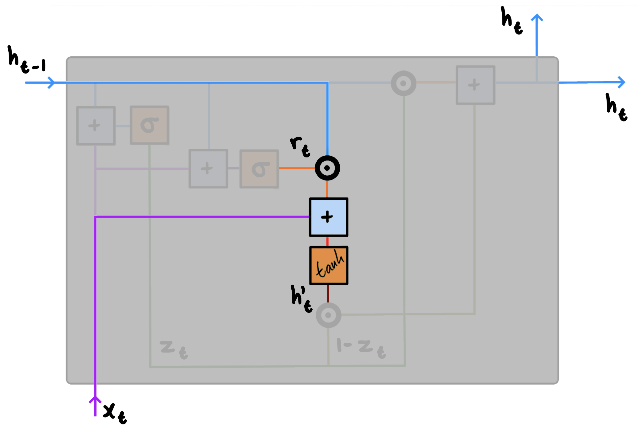
We compute the candidate activation $h’_t$ for time step $t$ using:

Specifically, we start by multiplying the input $x_t$ with weight $W$ and $h_{t-1}$ with weight $U$. We then compute the Hadamard—that is, element-wise—product between the reset gate $r_t$ and $Uh_{t-1}$. This step determines what should be forgotten from the previous steps. In machine translation tasks, for instance, towards the end of a sentence, most values in the $r_t$ vector are likely close to 0. We sum the results from both calculations and apply the $\tanh$ activation function. Note that if $r_t$ features low values, the reset gate effectively makes the unit act as though it is reading the first symbol of the input sequence. It is this mechanism which allows us to forget the previously computed state(s). The result of the $\tanh$ activation function is that all values are squashed between $-1$ and $1$. Additionally, since only zero-valued inputs are mapped to near-zero outputs, the elements the reset gate determined should be forgotten will, in effect, be forgotten here.

4. Activation

At the fourth and final step of our GRU, we need to compute the activation $h_t$, which is the vector containing the information describing the current state. In order to do this, we need to employ the output of the previous step alongside that of the update gate as to determine what information is relevant.

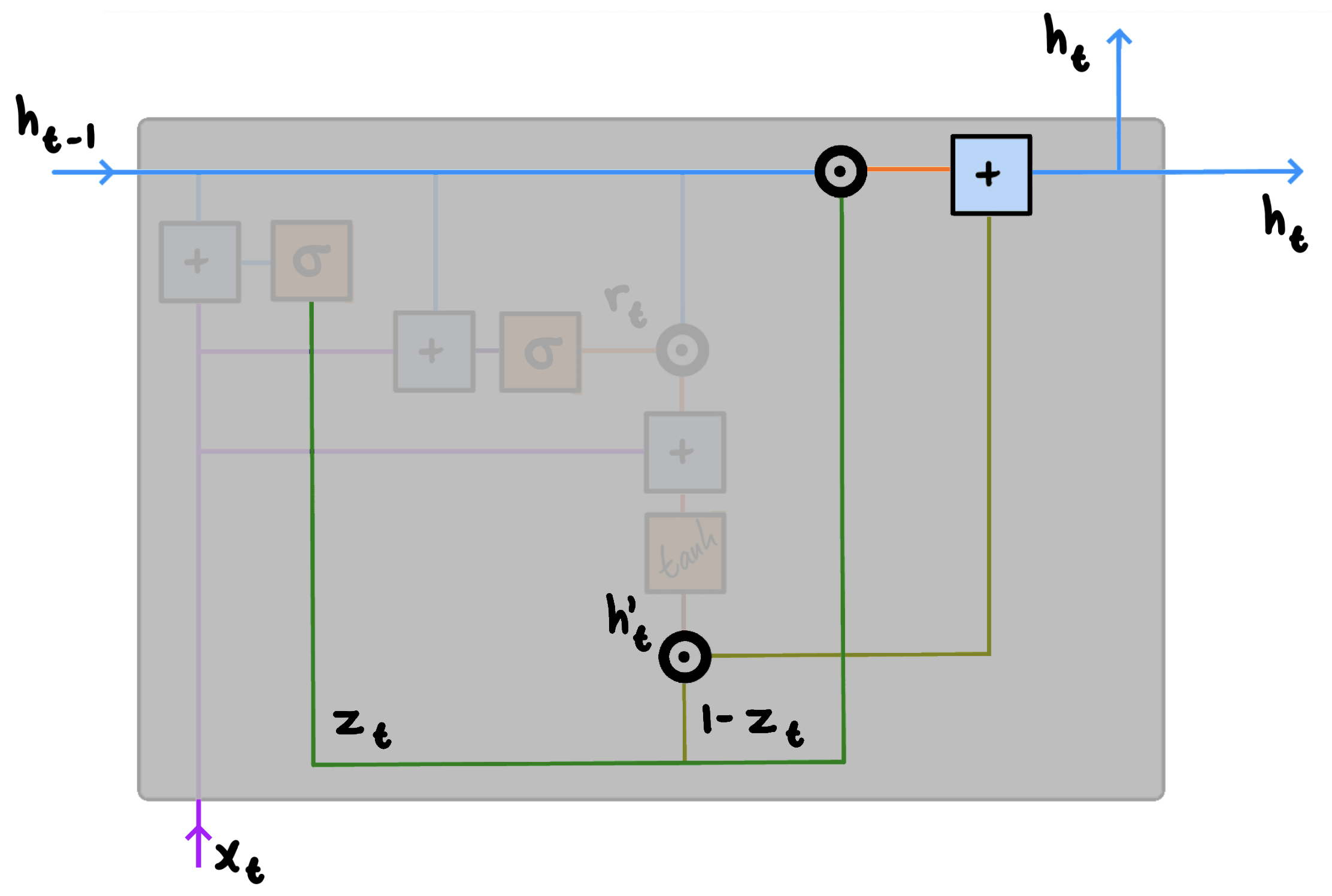
The activation $h_t$ is a linear interpolation between the previous activation, or previous hidden state, $h_{t-1}$ and the candidate activation $h’_t$. Specifically, we compute the activation $h_t$ for time step $t$ using:

We start by applying element-wise multiplication to the update gate $z_t$ and $h_{t-1}$. We then apply element-wise multiplication to $(1-z_t)$ and $h’_t$. The final result is obtained by summing the two intermediate results. The computed activation, or hidden state, $h_t$ can then be passed along to another GRU, an attention layer, or something else entirely. Note that since everything operates on individual time steps $t$, all of the above will happen for each individual element of the input sequence.

This is all that happens inside a GRU.

How do GRUs and LSTMs compare?

It is important to once again accentuate how both techniques seek to solve the same problem; namely that of the vanishing gradients. This makes both techniques relevant whenever dealing with data in which long-range dependencies are present (or perhaps merely suspected present). As such, it makes sense to briefly compare both solutions to conventional RNNs before comparing them directly: Indeed, shared by both GRUs and LSTMs is the additive component of their update from $t$ to $t+1$. This additive component does not exist in vanilla RNNs. Instead, vanilla RNNs replace the activation—that is, the content of the recurrent unit—with a value computed using only the current input and the previous hidden state. GRUs and LSTMs both retain the existing content and add more, new content on top. This has two distinct advantages. Namely, it (1) enables each unit to remember the existence of specific features from the input sequence; and (2) creates a shortcut of sorts, bypassing several temporal steps, and effectively enables the gradient to be backpropagated without quickly vanishing as a result of passing through multiple bounded non-linearities.

As previously mentioned though, one thing which GRUs are missing compared to LSTMs is the controlled exposure of the memory content. In a LSTM unit, the amount of memory content that is seen by other units in the network is controlled by a designated output gate. This gate does not exist in GRUs. Instead, all available information at each time step is always exposed in full. This can be both an advantage and a disadvantage depending on your data.

Another difference between the two techniques is the location of the input gate (in case of LSTMs) and the reset gate (in case of GRUs). In both cases, the job of the gate is the same. Notably, however, the input gate of LSTMs controls the amount of the new memory content that is being added to the memory cell independently from its forget gate. This is unlike GRUs in which the flow of information from previous activations is tied to the update gate, which alone determines how much passes through. Additionally, there is no dedicated memory cell in GRUs, though this does not necessarily mean that GRUs can remember less than LSTMs.

As you might have gauged by now, there is unfortunately no clear-cut answer when choosing whether to employ GRUs or LSTMs. Indeed, in most cases, either will do just fine. In some cases, depending on your data and the rest of your network, one might outperform the other ever so slightly. This, essentially, was the conclusion reached by Chung et al. [2014], who sought to empirically evaluate GRUs and LSTMs in the context of sequence modelling. Fortunately, both PyTorch and Tensorflow offer plug-n-play implementations of both, allowing you to experiment accordingly. In practice, swapping between GRUs and LSTMs is usually a matter of changing a couple of lines. What is worth noting is that since LSTMs have an additional gate and otherwise produce more output, it does require more memory and, as a consequence of having more parameters, might take longer to train.

It is conclusively important to stress that whilst GRUs and LSTMs have not exactly solved the problem of the vanishing gradients entirely, they have made it far more manageable. That is to say; given an input long enough, the vanishing gradients problem will eventually arise and alternative techniques such as attention are required.

Thanks for reading!
If this helped you, consider buying me a coffee!