
Introduction to Datalog
March 18, 2019
In contrast to the imperative programming paradigm, declarative programming expresses the logic of a computation without explicitly specifying its control flow. That is, declarative programming focuses on the what, not the how. If you have tentatively researched declarative programming before, you have likely read something akin to the above description already. If, on the other hand, this is your first time reading anything about declarative programming, the idea of developing an application without focusing on the how likely sounds alien – it sure did for me!
However, chances are that you have already worked declaratively without realising! Indeed, ubiquitous, domain-specific languages like HTML, CSS, and SQL all belong to the declarative paradigm. HTML, for instance, merely describes what should appear on a given webpage without regard to the order in which the various elements should be rendered by the browser. Similarly, a SQL query just describes what to return, not how to compute the return value. This, in essence, is what people mean when they say declarative programming focuses on the what.
It is worth accentuating how the term declarative programming is really an umbrella term which, in addition to the domain-specific languages mentioned above, also encapsulates the subparadigm logic programming. It is this particular subparadigm which we are going to concern ourselves with throughout this tutorial.
Logic programming is based on formal logic. This means that any program written in a logic programming language, e.g. Datalog or Prolog, is nothing more than a set of sentences in logical form, expressing facts and rules about a given domain. This allows logic programming to boast some nice features that other paradigms lack, namely:
- no side-effects,
- no explicit control flow, and
- strong guarantees about termination.
However, the fact that logic programming relies on sentences in logical form also affects its expressive power—that is, which algorithms can be expressed using which logic programming languages. The below illustration seeks to visualise this.
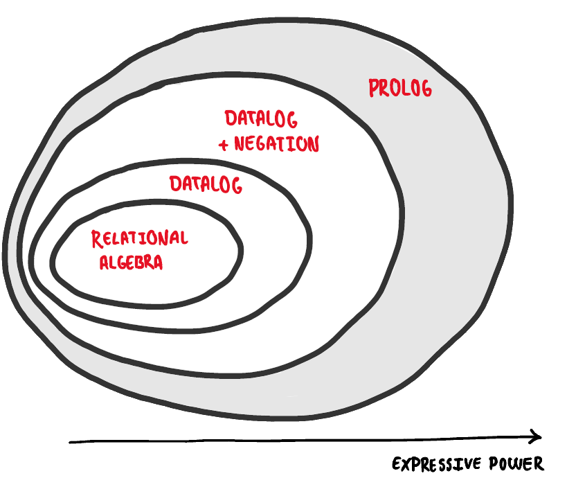
This is a simplified illustration, click here for more details.
The above illustration may be simple and easy to grasp, but it also incorrectly considers relational algebra a single concept. In reality, we differentiate between what is called positive relational algebra—the fragment of relational algebra which excludes the difference operator—and relational algebra. Any expression written in positive relational algebra, or $RA^{+}$, can be translated directly into a Datalog program, effectively making Datalog at least as expressive as $RA^{+}$. However, because Datalog can also express recursive queries, it is strictly more expressive than $RA^{+}$. There are, nonetheless, some expressions supported by relational algebra which cannot be expressed using Datalog; namely queries which employ the difference operator. These shortcomings are accommodated by Datalog with negation. This means a more accurate, though equally more complex, depiction of the expressive power would be the following:
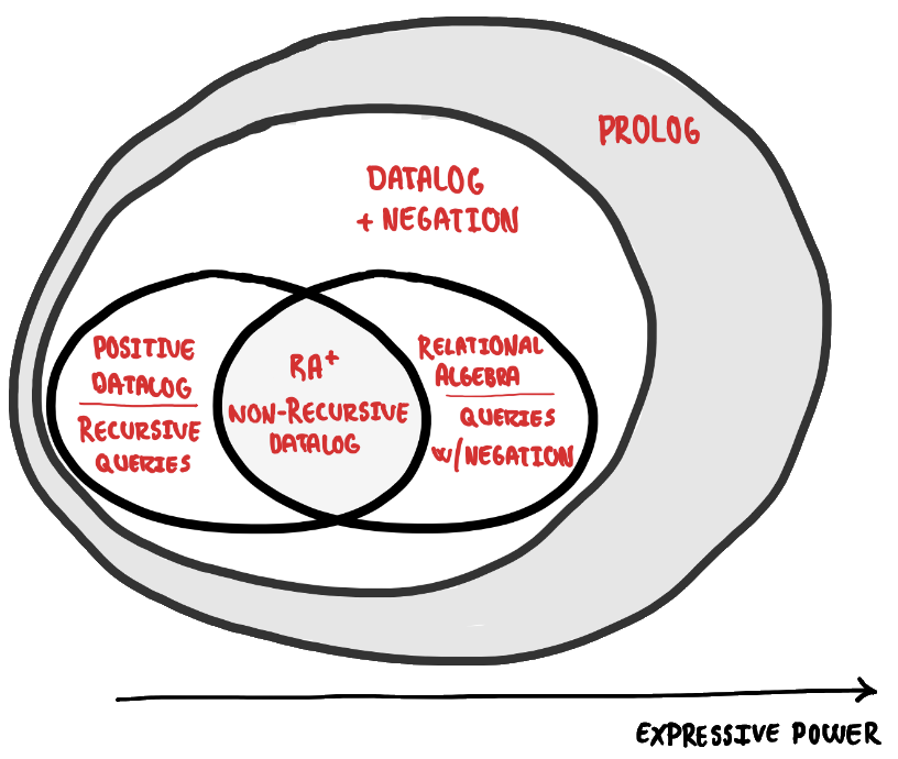
The innermost circle encapsulates relational algebra—something which you might be familiar with if you have SQL-experience—and shows Datalog as an immediate extension. We consider Datalog an immediate extension of relational algebra because whilst it, unlike relational algrebra, supports recursion, it can do little more. If you are unfamiliar with relational algebra there is no need to worry; we are not going to be writing any relational algebra in this tutorial. This is all about expressive power and putting things into perspective.
The next circle extends Datalog with negation. This allows us to implement any polynomial time algorithm using what is called stratified Datalog. It is worth noting that Datalog without negation, like relational algebra, is hardly useful in the real world. All references to Datalog will thus hereinafter refer to the version supporting negation unless explicitly stated otherwise. Indeed, if we take some precautions when extending Datalog with negation, we continue to retain strong guarantees about termination.
If we wish to express algorithms beyond those of polynomial time, however, we have to extend Datalog yet again. This time we move to the outermost circle, and thereby effectively transform Datalog to Prolog in the process. Prolog is a Turing-complete logic programming language which enables us to express any algorithm we so desire. As a direct consequence of this newly gained expressive power, however, we lose our nice guarantees about termination. I will briefly return to Prolog towards the end of this tutorial.
A new way of thinking
It is with the above in mind perhaps not surprising that Datalog, at its core, is a very simple language. The challenge with Datalog is thus not learning an extensive syntax, fighting your compiler, or juggling numerous libraries. The challenge, rather, lies, as with any new programming paradigm, in rewiring your brain to understand the concept. It is a new way of thinking!
We have already established how any program written in a logic programming language is written as a collection of logic constraints—that is, sentences in logical form. The compiler uses this collection of constraints to compute a solution. Read that again. Yes, really! In fact, the compiler can freely choose which algorithms and data structures to employ in order to compute a solution when prompted. We have no guarantees that the compiler will always choose the same approach, and it might even decide to do things in parallel! Given the same input, however, the compiler will always produce the same output. Fortunately, since the compiler takes care of this behind the scenes (the how), all we need to concern ourselves with is writing proper constraints (the what).
Facts and rules
All logic programs—that is, our collection of logic constraints—consist of a finite set of facts and rules, and Datalog programs are no exception. The concept of facts and rules is vaguely equivalent to that of classes and functions in other languages. In short:
- facts = assertions of the world in which we operate.
- rules = sentences allowing us to infer new facts from existing ones.
So far, so good… except, how do we actually write a Datalog program? Easy enough. We start by introducing some facts. Imagine, for instance, that we want to model our shelf with movies neatly organised by their main genres. This is straightforward:
Movie("Pulp Fiction", "Crime").
Movie("The Hateful Eight", "Crime").
Movie("Reservoir Dogs", "Thriller").
The above says that we have three facts, each holding two values and ended by a . (period). In this specific case, the two values are the title of the movie and the genre of the movie, respectively. The name—that is, the predicate—of each fact is Movie. If we then want to expand our world with, say, the actors from each movie:
StarringIn("Pulp Fiction", "Tim Roth").
StarringIn("The Hateful Eight", "Tim Roth").
StarringIn("Reservoir Dogs", "Harvey Keitel").
...
Similarly, if we want to include the name of the directors:
DirectedBy("Pulp Fiction", "Quentin Tarantino").
DirectedBy("The Hateful Eight", "Quentin Tarantino").
DirectedBy("Reservoir Dogs", "Quentin Tarantino").
And so on so forth!
It is generally a good idea to introduce your facts at the beginning of your program to enforce some concept of structure and order. However, if you prefer a different structure—perhaps you want things alphabetically—you can freely do so! Indeed, the lack of explicit control flow means that there is no pre-defined structure which you ought to obey. Additionally, when making facts, the order of your constants does not matter. That is:
DirectedBy("Reservoir Dogs", "Quentin Tarantino").
is as valid as
DirectedBy("Quentin Tarantino", "Reservoir Dogs").
You should thus simply opt for the approach which makes the most sense to you, and otherwise be consistent! The exact order of your constants only matters when writing rules, as we will see shortly.
Now, having modelled our movie collection, imagine a friend who really enjoys crime movies visits. They have a suspiciously specific preference in movies, and particularly appreciates movies directed by Quentin Tarantino starring Tim Roth. Which movie(s), then, should we put on?
We could obviously answer this by reading through the above facts, but imagine for a second that our movie collection spanned tens of thousands of titles—and thus exponentially more facts. Or, since few people are likely to have that many movies, imagine you are Netflix and need to recommend new movies based on what a given user has already expressed an interest in. The concept here is the same, and in both scenarios, opting for a manual approach quickly becomes mindbogglingly tedious, if not impossible.
Introducing rules!
ExtraAwesomeMovie(title) :-
    Movie(title, "Crime"),
    StarringIn(title, "Tim Roth"),
    DirectedBy(title, "Quentin Tarantino").
This rule reads as follows:
If there is a movie with title, and the genre of that title is
Crime, and the title starsTim Roth, and the title is directed byQuentin Tarantino.
We know we are dealing with a rule due to the :- part at the end of the first line. The :- represents material conditional with the left side being the consequent, and the right side being the antecedent. We read :- as “if”. Note that rules are checked against every available fact in our program, but only return the fact(s)—in this case movie(s)—for which the rule in question holds true. That is, we infer that a movie is an ExtraAwesomeMovie if and only if the above rule holds true.
If our example program had contained the fact FirstName("Jennifer")., this fact would, consequently, also have been checked in the above rule, but since there exists no Movie-fact with title “Jennifer” and genre “Crime”, the compiler would simply have continued to the next available fact. Of course, had there existed a Movie-fact with title “Jennifer” and genre “Crime”, it would still need to star Tim Roth and be directed by Quentin Tarantino to be returned.
Furthermore, whilst the order of our constants in our facts does not matter, we ultimately do need to obey the chosen order when writing rules. That is, Movie(title, "Crime") and Movie("Crime", title) are not the same! The first would with our set of facts match crime movies and return their titles, whereas the second would exclusively match movies called “Crime” and return their genres.
The result of the above ExtraAwesomeMovie-rule is:
ExtraAwesomeMovie("Pulp Fiction").
ExtraAwesomeMovie("The Hateful Eight").
The output above shows the two new facts of type ExtraAwesomeMovie which we have inferred from our original set of facts. Given the preferences of our friend which we used to design our rule, we can safely select either of the two movies since we know for a fact (pun intended!) that both are ExtraAwesomeMovie’s! Having introduced one example, we will now backtrack slightly and establish proper terminology and syntax.
Datalog Syntax
In Datalog, both facts and rules are represented as Horn clauses—the specifics of which we will not be covering in this post, though if the reader is interested, additional information may be found here. It is sufficient to know that a Horn clause is a clause which contains at most one positive literal, and that there exists three types of Horn clauses: (1) facts (or unit clauses), expressing unconditional knowledge, (2) rules, expressing conditional knowledge, and (3) goal clauses. We have already introduced the two former, and we will return to the third later.
The complete grammar of Datalog is:
\[\begin{matrix} P \in Program & = & c_1, ..., c_n \\ c \in Constraint & = & a_0 \Leftarrow a_1, ..., a_n \\ a \in Atom & = & p(t_1, ..., t_n) \\ t \in Term & = & k\enspace |\enspace x \end{matrix}\]Where
$p$ = finite set of predicate symbols.
$k$ = finite set of variable symbols.
$x$ = finite set of constants.
In other words: A Datalog program $P$ consists of a sequence of constraints $c_1, …, c_n$ – a design which means that the shortest possible Datalog program is the empty sequence of constraints. A constraint $c$ is a Horn clause consisting of a head atom $a_0$, and an optional sequence of body atoms $a_1, …, a_n$. If the body is empty, we are dealing with a fact, otherwise it is a rule. An atom $a$ consists of a predicate symbol—that is, a name—and a sequence of terms $t_1, …, t_n$. A term is either a constant (e.g. a string like "Crime", or an integer like 31), or a variable (e.g. title).
Or, explained visually:
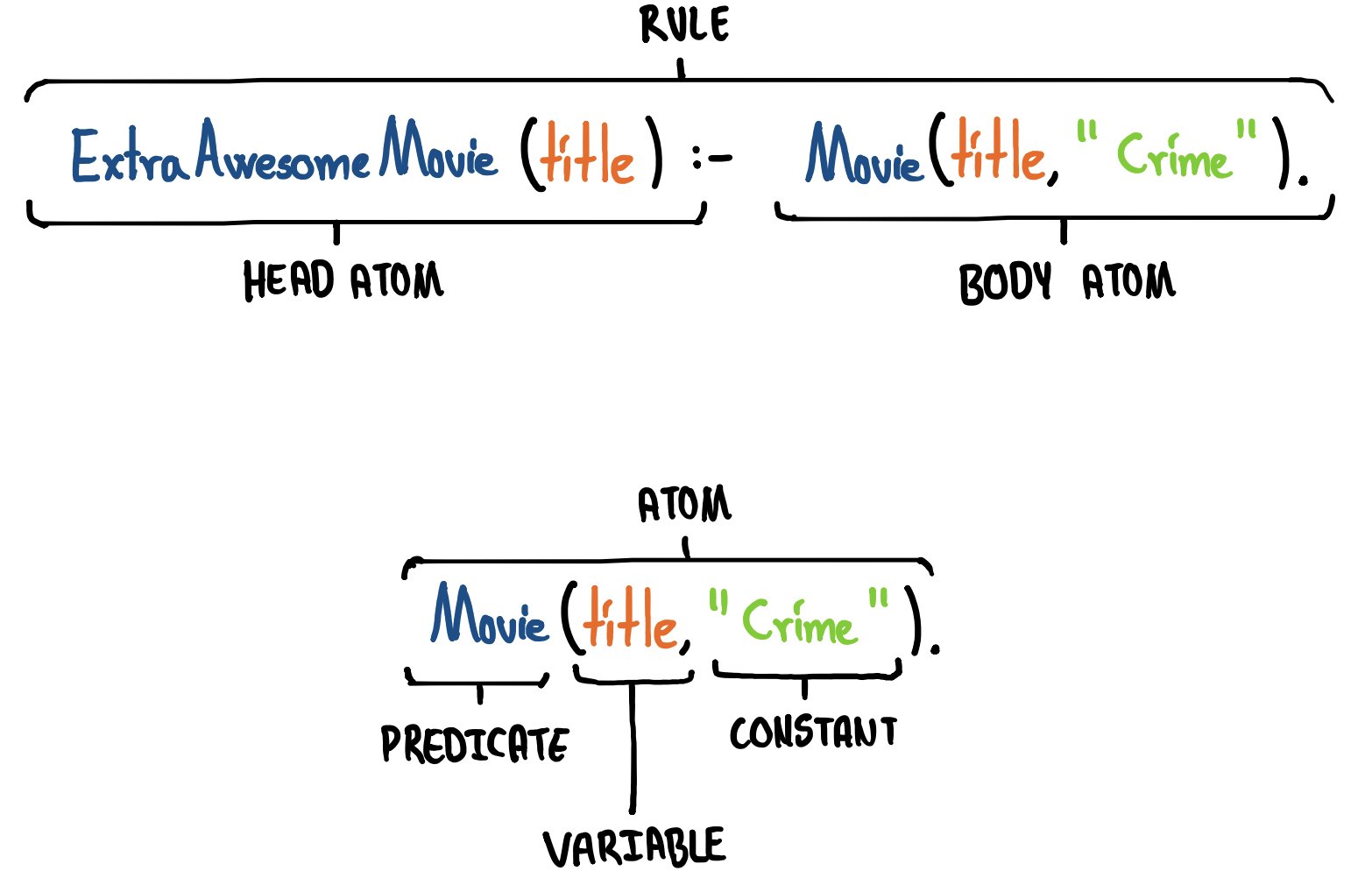
Additionally, as already noted, the . (period) at the end of a line concludes either that specific fact or rule. However, if we are writing a rule which contains multiple lines, we need to separate each but the last line using , (comma) as shown in the initial example above.
Different sources employ different terminology. Specifically, the concept of a constraint (which I refer to as either being a
factor arule) is also sometimes referred to as aclause, or justrule. Further, the concept of an atom is also sometimes referred to as aliteral. Some papers will mention which terminology they employ if it is not already obvious from the context.
This is it though. The above is the entire Datalog syntax.
Moving on!
Datalog Groundness and Safety
An atom is said to be ground if all its terms are constants, e.g:
NonGroundedFact("Walter White", actor).
is not grounded (due to the actor-variable), whereas
GroundedFact("Walter White", "Bryan Cranston").
is grounded because both terms are constants. Similary, a rule is said to be ground if all its atoms are grounded, for instance:
NonGroundedRule("Walter White", actor) :-
    MainCharacter("Walter White", "Breaking Bad"),
    StarringIn("Breaking Bad", actor).
is not grounded (due to the two actor-variables), whereas
GroundedRule("Walter White", "Bryan Cranston") :-
    MainCharacter("Walter White", "Breaking Bad"),
    StarringIn("Breaking Bad", "Bryan Cranston").
is grounded.
In order to ensure that we produce meaningful results, we introduce the notion of safety. We consider a given program $P$ safe iff every fact of $P$ is ground, and every variable $x$ that occurs in the head of a rule also occurs in the body of the rule (e.g. like how the actor variable in the abovementioned NonGroundRule appears both in the head and body). This is called the range restriction property.
It is important to accentuate that we do not need to have grounded rules for our Datalog program to be safe; we merely need to ensure that what appears in the head also at some point appears in the body at least once!
These conditions ensure that the set of facts which can be inferred from our Datalog program is finite—something which in turn guarantees that our program terminates. This is likely not something which you need to actively think about whilst programming considering how the vast majority of Datalog implementations outright reject unsafe programs, but now you know why rejection might happen!
Databases
We consider the facts in our program our database. We employ this database to answer queries—both by reading what is already in our database, and by using the existing knowledge to infer new knowledge liked we did with ExtraAwesomeMovie above. In the context of Datalog, a query is really just asking whether something exists one way or the other. We will return to queries in greater detail later.
In Datalog, we specifically operate with two distinct types of databases: (1) the extensional database (EDB), and (2) the intensional database (IDB). The EDB is the set of facts already in our Datalog program $P$, and the IDB is the set of facts we can infer from $P$. In other words, we can consider the EDB the input of our Datalog program, and the IDB the output of our Datalog program.
For instance, consider the program:
Edge("a", "b").
Edge("b", "c").

Path(x, y) :-
    Edge(x, y).

Path(x, z) :-
    Path(x, y),
    Edge(y, z).
The above Path-rule states that if there is a path from $x \rightarrow y$, and an edge from $y \rightarrow z$, then there is also an path from $x \rightarrow z$. At the moment, our EDB consists of two facts, namely:
Edge("a", "b").     extensional
Edge("b", "c").     extensional
However, by running the above program, we can infer three additional facts:
Edge("a", "b").     extensional
Edge("b", "c").     extensional

Path("a", "b").     intensional
Path("b", "c").     intensional
Path("a", "c").     intensional
Note how the output of a rule, in this case Path, consists of new ground atoms—facts—of the same name with terms satisfying the rule. The above should also make it clear why we can consider the EDB our input and the IDB our output. A Datalog program semantically is thus, in essence, an union between the EDB and the IDB.
What I refer to as “database” is also sometimes referred to as “schema”. That is, some papers operate with an “extensional schema” and an “intensional schema”. The abbreviations EDB and IDB, respectively, typically remain the same, however.
Datalog Semantics
In the introduction I alluded to the magic which transpires when the compiler computes a solution. It is not entirely true that we are completely in the dark when it comes to how the compiler operates. Indeed, there exists three different, equivalent Datalog semantics, namely:
- Model-theoretic semantics
- Fixed-point semantics
- Proof-theoretic semantics
These three semantics collectively hold a key to understanding Datalog programs. That is, by covering these three semantics, we attain the understanding and knowledge necessary to adequately reason about the solution of a Datalog program.
Model-theoretic semantics
Model-theoretic semantics define the meaning of a Datalog program in terms of interpretations and models. An interpretation is a set of facts, and a model is a specific interpretation which satisfy all constraints in our Datalog program. The smallest of such models is known as the minimal model, which is what we consider the solution. The intuition for model-theoretic semantics is that whilst a solution may be computed using different means, we can easily agree on the meaning of the query (e.g. find an
ExtraAwesomeMovie) as well as check whether a proposed solution is valid (e.g. if our friend is satisfied with the chosen movie).
To properly understand model-theoretic semantics, we need to introduce some additional definitions and concepts:
- Herbrand Universe
- Herbrand Base
- Truth
- Models
- Minimality
To assist our understanding of the above, consider the program:
Parent("Sansa Stark", "Eddard Stark").
Parent("Arya Stark", "Eddard Stark").
Parent("Eddard Stark", "Rickard Stark").

GrandParent(x, z) :-
    Parent(x, y),
    Parent(y, z).
The Herbrand Universe, $U$, is the set of all constants appearing anywhere in our program. Note that if some constants are introduced in a rule, these, too, will be included in $U$. In the above example,
$U$ = {"Sansa Stark, "Arya Stark", "Eddard Stark", "Rickard Stark"}.
The Herbrand Base, $B$, is the set of all ground atoms with predicate symbols drawn from our program and terms drawn from the Herbrand Universe $U$. Intuitively, we can think of $B$ as the EDB (the existing facts), the IDB (the facts we can infer), and the un-inferrable facts (meaningless facts) all mixed together.
Consider $B$ of the above example:
Parent("Arya Stark", "Arya Stark").         GrandParent("Arya Stark", "Arya Stark").
Parent("Arya Stark", "Sansa Stark").        GrandParent("Arya Stark", "Sansa Stark").
Parent("Arya Stark", "Eddard Stark").       GrandParent("Arya Stark", "Eddard Stark").
Parent("Arya Stark", "Rickard Stark").      GrandParent("Arya Stark", "Rickard Stark").
Parent("Sansa Stark", "Sansa Stark").       GrandParent("Sansa Stark", "Sansa Stark").
Parent("Sansa Stark", "Arya Stark").        GrandParent("Sansa Stark", "Arya Stark").
Parent("Sansa Stark", "Eddard Stark").      GrandParent("Sansa Stark", "Eddard Stark").
Parent("Sansa Stark", "Rickard Stark").     GrandParent("Sansa Stark", "Rickard Stark").
Parent("Eddard Stark", "Arya Stark").       GrandParent("Eddard Stark", "Arya Stark").
Parent("Eddard Stark", "Sansa Stark").      GrandParent("Eddard Stark", "Sansa Stark").
Parent("Eddard Stark", "Eddard Stark").     GrandParent("Eddard Stark", "Eddard Stark").
Parent("Eddard Stark", "Rickard Stark").    GrandParent("Eddard Stark", "Rickard Stark").
Parent("Rickard Stark", "Arya Stark").      GrandParent("Rickard Stark", "Arya Stark").
Parent("Rickard Stark", "Sansa Stark").     GrandParent("Rickard Stark", "Sansa Stark").
Parent("Rickard Stark", "Eddard Stark").    GrandParent("Rickard Stark", "Eddard Stark").
Parent("Rickard Stark", "Rickard Stark").   GrandParent("Rickard Stark", "Rickard Stark").
You will quickly notice how, as already hinted, many of the above atoms make absolutely no sense; e.g. GrandParent("Arya Stark", "Arya Stark").. This is why we need to reintroduce the notion of interpretations. As already mentioned, an interpretation is a set of facts. More specifically, however, a given interpretation is a subset of the Herbrand Base.
An interpretation is also sometimes referred to as a database instance.
For example,
Parent("Rickard Stark", "Eddard Stark").    GrandParent("Rickard Stark", "Eddard Stark").
Parent("Rickard Stark", "Rickard Stark").   GrandParent("Rickard Stark", "Rickard Stark").
is an interpretation. However, as should be evident, not every interpretation is going to be true. This does not mean that we cannot say anything about the truth given an interpretation, though! Remember, all the correct facts are also part of our Herbrand Base. Given any interpretation $I$, we can determine the truth of a constraint as follows:
- A ground atom $a = p(k_1, …, k_n)$ is true for $I$ if $a \in I$.
- A conjunction of atoms, $a_1, …, a_n$ is true for $I$ if each $a$ is true in $I$.
- A ground rule $a_0 \Leftarrow a_1, …, a_n$ is true for $I$ if either the body conjunction is false, or the head atom is true.
That is, given an interpretation $I$:
Parent("Arya Stark", "Eddard Stark").
Parent("Eddard Stark", "Rickard Stark").
GrandParent("Arya Stark", "Rickard Stark").
The ground atom
Parent("Arya Stark", "Eddard Stark").
is true because it appears in $I$. However, the ground atom
Parent("Sansa Stark", "Eddard Stark").
is false because it does not appear in $I$. Again, this does not mean the fact itself is wrong; we are exclusively considering this in the context of the given interpretation.
The ground rule
GrandParent("Arya Stark", "Rickard Stark") :-
    Parent("Arya Stark", "Eddard Stark").
    Parent("Eddark Stark", "Rickard Stark").
is true. Why? Again, for rules, either the body is false, or, if the body is true, the head has to be true. The first Parent atom (Parent("Arya Stark", "Eddard Stark")) is in $I$—as is the second Parent atom (Parent("Eddard Stark", "Rickard Stark")). This means that the body is true, which means the head ground atom must be in the interpretation $I$, which it is. In other words, given the above interpretation $I$, the above ground rule is true.
Just because an interpretation is true does not mean it is also true in the real world. It is important to accentuate how the notion of truth is wholly reliant on the specific domain which we have modelled and operate in. Incorrect data will, therefore, inherently, lead to incorrect answers—much like how a tainted SQL database will result in incorrect or misleading answers.
This leads us to the notion of models. In short, a model $M$ of a Datalog program $P$ is an interpretation $I$ that makes each ground instance of each rule in $P$ true. A ground instance of a rule is obtained by replacing every variable in a rule with a constant from the Herbrand Universe.
In our above example, this would translate to the interpretation:
Parent("Arya Stark", "Eddard Stark").
Parent("Sansa Stark", "Eddard Stark").
Parent("Eddard Stark", "Rickard Stark").
GrandParent("Arya Stark", "Rickard Stark").
GrandParent("Sansa Stark", "Rickard Stark").
In other words, a model is an interpretation for which when we instantiate all ground rules in our program, they are satisfied by the set of facts in the interpretation.
A model $M$ is minimal if and only if there is no other model which contains fewer facts. What this means is that the minimal model is the intersection of all models. A direct consequence hereof is that the minimal model is unique. This is what allows any Datalog program to always have a unique solution—the minimal model.
In short, model-theoretic semantics allows us to check a given solution and verify whether it is the minimal model. We first confirm whether all ground rule instances are true, and then, if they are, we know we have a model. We then check to see if that model is minimal by checking whether any facts can be removed.
A natural question, then, is how do we actually find the minimal model?
Fixed-point semantics
Using the above principles of model-theoretic semantics, we develop a method for finding the minimal model. We start by defining the notion of an immediate consequence operator, $T_p$, as the head atoms of each ground rule instance satisfied by a given interpretation $I$. That was quite a mouthful, so consider the following interpretation from our Game of Thrones inspired example instead:
Parent("Arya Stark", "Eddard Stark").
Parent("Eddard Stark", "Rickard Stark").
The above facts satisfy our GroundParent-rule and allows us to ground it:
GrandParent("Arya Stark", "Rickard Stark").
We now have a new fact which we can continue working with. $T_p$ can intuitively be thought of as iteratively computing the set of facts which can be inferred in a single step from a given interpretation $I$. Or, in other words:
\[\begin{matrix} Iteration0& = & T_p(Ø)\\ Iteration1& = & T_p(T_p(Ø))\\ Iteration2& = & T_p(T_p(T_p(Ø)))\\ ... & = & ... \\ Iteration_{n} & = & T_p^{n}(Ø) \end{matrix}\]Where $Ø$ is empty set of facts and where $Iteration0$ translates to our EDB—that is, the facts already in your program. Please note how $T_p^{2}(Ø) = T_p(T_p(Ø))$, which is why it suffices to write $Iteration_{n}$ the way we do above. What really happens above though is that we repeatedly apply $T_p$ to itself starting from the empty set. We continue to do this until we stop inferring new facts. This process is called computing the least-fixed point of $T_p$.
Consider this example:
Edge("a", "b").
Edge("b", "c").
Edge("c", "d").
Edge("d", "e").

Path(x, y) :-
    Edge(x, y).

Path(x, z) :-
    Path(x, y),
    Edge(y, z).
$Iteration0$ =
// facts                iteration
Edge("a", "b").         0
Edge("b", "c").         0
Edge("c", "d").         0
Edge("d", "e").         0
Now we have the four edges which appear in the program itself. We cannot use the second Path-rule because that requires both a path and an edge. We can, however, use the first Path-rule, so we will do just that.
$Iteration1$ =
// facts                iteration
Path("a", "b").         1
Path("b", "c").         1
Path("c", "d").         1
Path("d", "e").         1
We now have four edges and four paths. We can now use the second Path rule to infer even more paths.
$Iteration2$ =
// facts                iteration
Path("a", "c").         2
Path("b", "d").         2
Path("c", "e").         2
And again, with the new paths.
$Iteration3$ =
// facts                iteration
Path("a", "d").         3
Path("b", "e").         3
And again.
$Iteration4$ =
// facts                iteration
Path("a", "e").         4
At this point we have exhausted how many new facts we can infer, and we have a final result. Notice that any further application of the $T_p$-function will not alter the result—meaning that we have reached the fixed-point, hence the name. A fixed-point for a function $f$ is a value $x$, such that $f(x) = x$. Additional information about fixed-point arithmetics can be found here.
// facts                iteration
Edge("a", "b").         0
Edge("b", "c").         0
Edge("c", "d").         0
Edge("d", "e").         0
Path("a", "b").         1
Path("b", "c").         1
Path("c", "d").         1
Path("d", "e").         1
Path("a", "c").         2
Path("b", "d").         2
Path("c", "e").         2
Path("a", "d").         3
Path("b", "e").         3
Path("a", "e").         4
The above is the minimal model of our program.
Using the immediate consequence operator to compute the minimal model of a given Datalog program is called bottom-up evaluation. This description makes sense when considering how we start from nothing—the empty set of facts—and iteratively move up by computing new facts using the previous ones. The example covered here employs a strategy called naïve evaluation, though a better, far more efficient strategy used in practice is called semi-naïve evaluation. The essential idea of this approach is to keep track of the inferred facts and only re-evaluate the rules affected by the new facts using only the new facts. We will not be covering the specifics as it is sufficient to know that this approach exists (your Datalog engine most likely uses it!), and what bottom-up evaluation is in general.
Proof-theoretic semantics
So far, so good. However, what if we only really want to know whether there exists a path from $a \rightarrow d$? We could naturally compute all paths in the program, like we just did, and check once done. This is fine, but it is not really super optimal either! Proof-theoretic semantics seeks to solve (read: optimise) this. We can now, finally, properly introduce the third type of Horn clauses previously mentioned; goals.
A goal is also sometimes called a “query”, which makes sense when discussing its practical usage as I have done thus far. However, in the context of this section, I will opt for using the goal-term. You may use them interchangeably, though.
A goal is an atom which we want to determine whether exists in the minimal model. A goal can be ground or have free variables—in the case of the latter, we would want to determine the values of those variables before returning. Where we end facts and rules with a . (period), goals are ended with a ? (question mark) as though we were posing a question—which, in many ways, is exactly what we are! The output of a goal is both a simple true / false answer, but also a proof tree which shows how the goal was actually inferred. Because of the proof tree, proof-semantic semantics is called top-down evaluation.
If we return to our previous example once again:
Edge("a", "b").
Edge("b", "c").
Edge("c", "d").
Edge("d", "e").

Path(x, y) :-
    Edge(x, y).

Path(x, z) :-
    Path(x, y),
    Edge(y, z).
And say we want to know whether there exists a path $a \rightarrow d$?. In practice, the query would be Path("a", "d")?, though this might differ slightly depending on your Datalog engine (some handle queries as filters, for instance). In the above program, however, we have two means of deriving a path; either
// rule 1
Path(x, y) :-
    Edge(x, y).
or
// rule 2
Path(x, z) :-
    Path(x, y),
    Edge(y, z).
If we then insert our "a" and "d", we get
// rule 1
Path("a", "d") :-
    Edge("a", "d").
and
// rule 2
Path("a", "d") :-
    Path("a", y),
    Edge(y, "d").
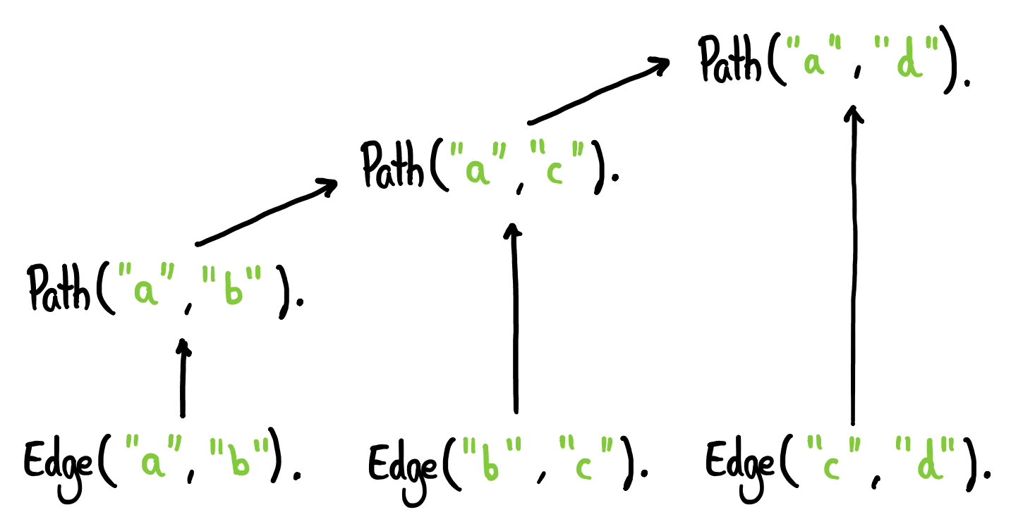
The first rule can obviously not be used; we have no Edge("a", "d").. However, the second rule can be used. Indeed, since the second rule initially contains three variables, we now effectively have two subgoals, namely:
Path("a", y)?
Edge(y, "d")?
Notice how the above two subgoals are taken directly from the body of the second rule. Of these, the second subgoal, Edge(y, "d")?, is quickly solved by checking our EDB: We have an Edge(y, "d"). if y = "c". This leaves just one subgoal. However, since we just solved Edge(y, "d")? as Edge("c", "d")., we need to replace y with "c" in the remaining subgoal as well because this, too, relies on y. We thus recurse once again, seeking this time to derive Path("a", "c")?:
// rule 1
Path("a", "c") :-
    Edge("a", "c").
The first rule is, once again, useless, so we immediately turn our attention to the second rule:
// rule 2
Path("a", "c") :-
    Path("a", y),
    Edge(y, "c").
… and so on, so forth.
The ultimate output, beyond a true / false to our initial goal or query, is a proof-tree as illustrated below:
Datalog with Negation
We have now established how to determine whether a specific path exists. However, what if what we are really interested in finding is the set of pairs for which there is no path from $x \rightarrow y$? Introducing negation! If you recall the very first illustration, we are now moving to the third innermost circle, just below Prolog.
As an example, let us update our previous path program:
Vertex("a").
Vertex("b").
Vertex("c").
Vertex("d").
Vertex("e").
Edge("a", "b").
Edge("b", "c").
Edge("c", "d").

Path(x, y) :-
    Edge(x, y).

Path(x, z) :-
    Path(x, y),
    Edge(y, z).

Unconnected(x, y) :-
    Vertex (x),
    Vertex (y),
    not Path(x, y).
The above Unconnected rule reads if there is a vertex x, and a vertex y, and there is no path from x $\rightarrow$ y. However, before we proceed, we need to update our grammar to properly accommodate negation. It is a minor change as we really only need to distinguish between head and body atoms, as well as allow atoms in the body to be negated.
The complete grammar of Datalog with negation is:
\[\begin{matrix} P \in Program & = & c_1, ..., c_n \\ c \in Constraint & = & a_0 \Leftarrow b_1, ..., b_n \\ a \in HeadAtom & = & p(t_1, ..., t_n) \\ b \in BodyAtom & = & p(t_1, ..., t_n) \\ & | & not\enspace p(t_1, ..., t_n)\\ t \in Term & = & k \enspace | \enspace x \end{matrix}\]Where
$p$ = finite set of predicate symbols.
$k$ = finite set of variable symbols.
$x$ = finite set of constants.
This change also means we need to update our notion of truth with regards to a given interpretation. Given an interpretation $I$, we now determine the truth of a constraint as follows:
- A positive ground atom $b$ is true for $I$ if $b \in I$.
- A negative ground atom $b$ is true for $I$ if $b \notin I$.
- A conjunction of atoms, $b_1, …, b_n$ is true for $I$ if each $b$ is true in $I$.
- A ground rule $b_0 \Leftarrow a_1, …, b_n$ is true for $I$ if either the body conjunction is false, or the head atom is true.
Note how the only change is distinguishing between positive and negative atoms.
Problems with negation
Nothing is ever simple.
Consider the program:
Actor(x) :- not Actress(x).
Actress(x) :- not Actor(x).
Assume that the Herbrand Universe, $U$, is the constant "Alex". In such a scenario, the above program has two “minimal” models, namely: $M_1 = {Actor(“Alex”)}$ and $M_2 = {Actress(“Alex”)}$. If we look at $M_1$ first, and replace the variable x with a constant from $U$, we have as our first rule:
Actor("Alex") :- not Actress("Alex").
Since Actress("Alex"). does not exist in $M_1$, the body atom is true. This, as per the rules regarding truth above, must mean that the head atom is true—that is, Actor("Alex"). must be true.
If we then look at the second rule:
Actress("Alex") :- not Actor("Alex").
Since Actor("Alex"). is in $M_1$, the body of the Actress-rule is false. However, since a false body does not say anything about the head, we effectively conclude that $M_1$ is a valid model. Following this logic, we can also conclude that $M_2$ is a valid model. This is a problem because neither of the two is the minimal model—there can, by definition, only be one minimal model!
Stratified negation
If we disallow recursion through negation, we can circumvent the abovementioned issues whilst still accommodating negation. In essence, the idea is to separate our Datalog program $P$ into a sequence of smaller, more confined programs $P_{1}, …, P_{n}$, and then compute them one by one as such:
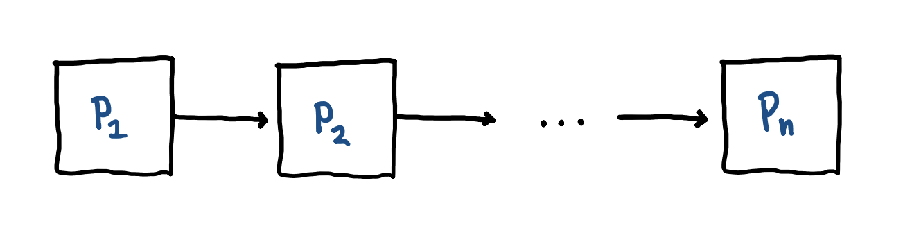
The arrow symbolises how the computed facts—the IDB $\cup$ EDB—of a given subprogram $p_{i}$ becomes the facts—the EDB—of the next subprogram $p_{i+1}$. The solution will then be the facts computed by the final subprogram, $p_{n}$.
A stratification of a Datalog program $P$ is a partition of the predicate symbols subject to the following two conditions: If there is a rule
(1) $A(…) \Leftarrow …, B(…), …$ in $P$, where the predicate $A$ is in stratum $p_{i}$, and the predicate $B$ is in stratum $p_{j}$, then $i \geq j$.
(2) $A(…) \Leftarrow …, not \enspace B(…), …$ in $P$ where the predicate $A$ is in stratum $p_{i}$, and the predicate $B$ is in stratum $p_{j}$, then $i > j$.
If we look at the second rule, what this really says is that in order to compute $A$, we must know what $B$ is. In other words: $B$ must belong to a lower strata such that it can be completely computed before we attempt to compute $A$. It is in this regard worth noting that it is possible to write programs which do not obey the above two rules. These programs need to be rejected, and most Datalog engines will do so accordingly. In conclusion though, a given Datalog program $P$ is said to be stratifiable if it has a stratification (and thus obeys the above two rules). Once we have a stratified Datalog program, it must satisfy an additional safety property, namely: Every variable which occurs in a negative atom must also occur in a positive atom in the body.
That is, the following
Unconnected(x, y) :-
    not Path(x, y).
is considered unsafe because x and y are not positively bound, whereas
Unconnected(x, y) :-
    Vertex(x),
    Vertex(y),
    not Path(x, y).
is safe because the two negated variables appear in positive atoms in the body. This means that if we look at our Datalog program once again:
Path(x, y) :-
    Edge(x, y).

Path(x, z) :-
    Path(x, y),
    Edge(y, z).

Unconnected(x, y) :-
    Vertex (x),
    Vertex (y),
    not Path(x, y).
We can stratify it by partitioning it as such:
$p_{0}$ = {$Edge, Path, Vertex$}
$p_{1}$ = {$Unconnected$}
The reason why we partition as above—and in the process ensure we can compute a minimal model—is that $Unconnected$ is the only rule in which negation is employed. It is, moreover, evident that we need to know what $Path$ is before we can say anything about what $Path$ is not. This is fortunately possible; as is saying something about $Edge$ and $Vertex$. As already alluded to, however, we have no guarantee that a given Datalog program is actually stratifiable… so how we do determine whether that is the case?
Precedence graphs
Given a Datalog program $P$, we define the precedence graph $g$ as follows. If there is a rule:
- $A(…) \Leftarrow …, B(…), …$, then there is an edge $B \xrightarrow{} A$.
- $A(…) \Leftarrow …, not \enspace B(…), …$, then there is an edge $B \xrightarrow{-} A$.
A Datalog program is stratifiable iff its precendece graph contains no cycles labelled with $-$. This means that even if we had a massive precedence graph with thousands of edges forming a cycle, if just one of the edges had a $-$ label, the Datalog program would not be stratifiable. In most cases, it will be possible to rewrite the program in such a manner that the meaning and inteded result are preserved.
Consider the program:
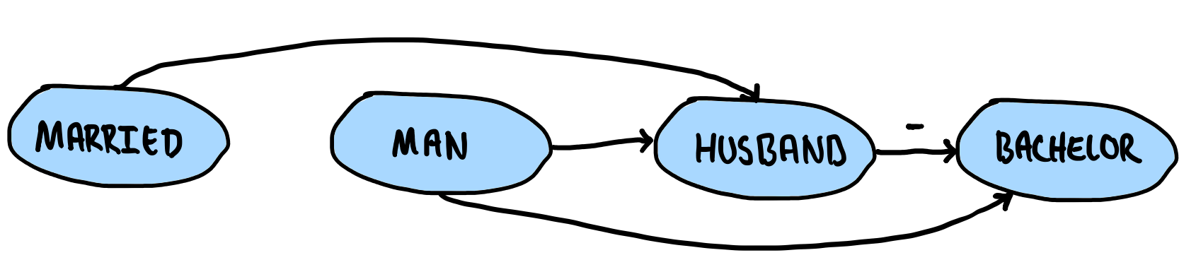
Husband(x) :-
    Man(x),
    Married(x).

Bachelor(x) :-
    Man(x),
    not Husband(x).
A Man is a Bachelor if he is not a Husband, and a Man is a Husband if he is Married. If we then draw the precedence graph of this program, we get:
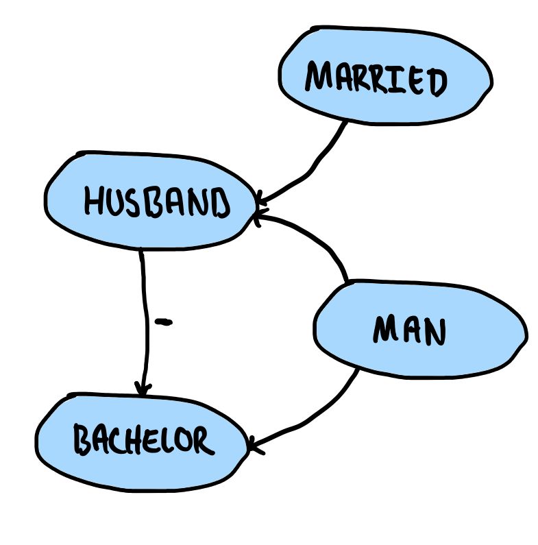
This seems fine; no cycles with a negated edge! If, on the other hand, our program looked like
Husband(x) :-
    Man(x),
    not Bachelor(x).

Bachelor(x) :-
    Man(x),
    not Husband(x)
and we now consider a Husband a Man who is not a Bachelor, and a Bachelor a Man who is not a Husband, our precedence graph would look as follows:
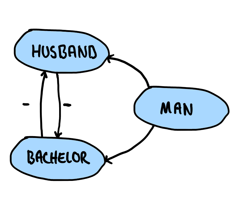
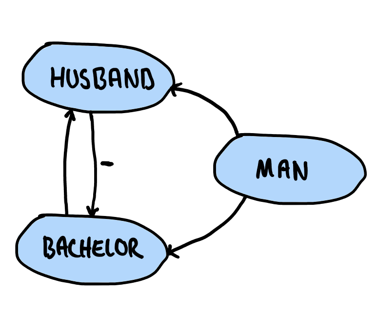
Observe how we now have a cycle with a negated edge. This version of our program is, consequently, not stratifiable. It is important to accentuate that there need not be a $-$ on every edge in the cycle for the program to not be stratifiable. Indeed, the following precedence graph would be equally problematic:
With a proper precedence graph $g$ in hand, we can compute the strata by first computing the strongly connected components of $g$ and then conducting a topological sort of these components. The order of the strata for the above program, for instance, would be:
Indeed, since Married and Man are independent, we can start with those two. However, because the first rule states $i \geq j$, we can also include Husband in this partition. That is, $p_{0}$ = {$Married, Man, Husband$}. Unlike every other node, Bachelor depends on what Husband is not. We thus need to know what Husband is first before we can say what it is not—note how the second rule states $i > j$. This makes $p_{1}$ = {$Bachelor$}. Each partition corresponds to a different strata.
Prolog
Prolog is like Datalog, but features two, seemingly simple extensions; (1) a fact may contain variables, and (2) a term may be a function application. However simple these changes might appear, the impact is profound. Prolog is a Turing-complete language, but it lacks some of Datalog’s neat properties, namely:
- No termination guarantee
- No (finite) minimal model
- No fixed-point semantics
This means that where we in Datalog deterministically can enumerate all facts with a bottom-up evaluation, or search for a specific fact using top-down evaluation, we are limited to searching with top-down evaluation without guarantees of termination in Prolog. However, on the other hand, Prolog now offers all the expressive power we need to express any given algorithm! There are many strategies one can employ whilst programming in Prolog to avoid most pitfalls, though unlike Datalog, these now need to be actively accounted for.